Towards Unified Models for Explainable AI in Precision Medicine
Cross-scale consistency from biological trajectories to clinical outcomes
Rui Miao
Department of Mathematical Sciences Texas AI Research Institute University of Texas at Dallas
Opening
Prediction is not enough.
Fragmented workflow
Biology, trajectory, and survival are modeled separately.
Explanations are added after prediction.
Clinicians see a scalar risk score without a disease story.
Unified workflow
Scale means the resolution of representation: covariates, latent state, trajectories, and outcomes.
One representation is constrained by multiple clinical observables.
Explanations interrogate both raw features and latent organization.
Validation asks whether all layers agree.
Explainability should be evaluated by cross-scale coherence, not by a single post hoc feature-importance plot.
Use case
Sickle cell disease is an ideal stress test for unified explainable AI.
Why this disease exposes the modeling problem
SCD has complicated heterogeneous progression across hematologic, renal, hepatic, and cardiopulmonary systems.
Those progression patterns are associated with survival outcomes, not just cross-sectional severity.
Mortality is clinically decisive but statistically sparse and censored.
The modeling target is heterogeneous disease progression linked to outcome, not a treatment-response claim.
Use case
The statistical problem is not "more variables"; it is missing supervision.
Rare observed events
Mortality is decisive but sparse, censored, and noisy at fixed horizons.
Composite endpoint burden
A single event label is hard to explain biologically without progression anchors.
Weak supervision
Baseline risk models need additional structure to learn disease state.
Prediction-time constraint
Risk must be computable from baseline variables alone for counseling, triage, and advanced-therapy decisions.
Training-time opportunity
Early biomarker trajectories are available during model development and provide progression supervision for the latent state.
Key design: longitudinal biomarkers shape the representation during training, but are not required at inference.
Data
Data setting: NHLBI adult SCD cohorts
Main cohort
adults
598
deaths
218
5y mortality
16.5%
Median follow-up 7.1 years. Rich baseline labs and echocardiography plus auxiliary longitudinal biomarkers.
Validation cohort
adults
383
deaths
42
5y mortality
22.9%
Median follow-up 2.2 years. Used only for external validation, not for model fitting or selection.
Footnote: main and validation analytic cohorts are drawn from NHLBI protocols 01-H-0088 and 04-H-0161 but are different cohorts; auxiliary trajectories are available only in the main cohort.
Data
Three data anchors: baseline profile, auxiliary trajectories, and survival
Baseline patient profile
68 baseline covariates.
demographicsgenotypelabsechocardiographyvitals
Auxiliary longitudinal supervision
12 biomarkers over a 3-year window, observed irregularly and restricted to early follow-up.
renalhepaticcardiopulmonaryphysiology
Survival endpoint
All-cause mortality with censoring provides the hard clinical outcome.
death eventcensoring5-year risk15-year risk
Framework
Cross-scale consistency: the central object of the talk
Biological
Labs and echocardiography proxy organ-level pathophysiology.
Temporal
The same latent state should support short-term biomarker evolution.
Outcome
It should support calibrated long-horizon survival prediction.
Interpretive
Feature, subject, and latent-phenotype explanations should agree.
Do not draw \(y\) as the next coarse-grained state. \(z_i\) is the shared state; trajectory reads from \(z_i\), while survival first passes through \(z_i^S\).
Framework
Renormalization Group is a disciplined analogy, not a literal claim.
Physics example: 2D Ising block-spin RG
Clinical analogy: readouts attach at the right scale
Framework
Patient-level coarse-graining: from clinical measurements to an effective disease state
Some progression readouts can attach to intermediate layers \(h_i^{(k)}\). The survival-specific state \(z_i^S\) is a coarser downstream layer for mortality risk.
The observable \(\hat y_{ik}(t)\) is not itself the next coarse-grained state; it is a readout from whichever hidden layer best carries that biological scale.
Framework
Residual stream and RG: the analogy is an evolving effective patient state.
Skip connection preserves the previous state; the residual block adds a task-guided correction; LayerNorm stabilizes the updated state.
Clinical-biological interpretation
The residual stream is not physical RG. It is the network's running effective patient state. Each block rewrites the representation while preserving what matters for trajectory and survival observables.
Framework
LayerNorm is the stabilizing step after each residual correction.
\(\mu_i\) and \(\sigma_i\) are computed across hidden coordinates within subject \(i\), not across patients. \(\gamma_\ell\) and \(\beta_\ell\) are learned.
This normalizes one subject's internal hidden vector, not one clinical covariate across the cohort.
Framework
Trajectory reads from shared z; survival reads from a survival-specific latent state.
For the SCD model used here, this is the simplified case: all 12 trajectory heads read from the last hidden layer \(z_i=h_i^{(L)}\); survival then reads from \(z_i^S\).
The losses define relevance: survival preserves event-time discrimination and calibration; trajectories preserve short-term biological progression.
Model
Model architecture: shared representation, task-specific heads
One shared patient state supports trajectory prediction; the survival branch then applies its own latent processing state before producing mortality risk.
Model
Missingness and validation logic are part of the model design.
Missingness handling
Random forest imputation separately for main and validation cohorts.
Missingness indicators enter the attention encoder.
Random missingness masks improve robustness.
Longitudinal timestamps are preserved.
Validation logic
C-statistic for discrimination.
5-year Integrated Brier Score for prediction error.
Simulated 10-30% missingness without retraining.
Validation cohort untouched during fitting and selection.
Results
Central ablation: trajectory-supervised survival improves discrimination and prediction error.
Main cohort
Model
C-stat
5y IBS
TSML (Sachdev 2021)*
0.739
0.058
Single-task DeepHit
0.827
0.037
Multi-Task DeepHit
0.882
0.029
TSML Sachdev 2021
Single-task
Multi-task
External validation
Model
C-stat
5y IBS
TSML (Sachdev 2021)*
0.661
0.085
Single-task DeepHit
0.747
0.072
Multi-Task DeepHit
0.794
0.064
The important ablation is not "deep learning vs statistics"; it is baseline-only survival vs baseline-only survival constrained by trajectory supervision.
* TSML benchmark from Sachdev V. et al. 2021; TSML = two-step machine learning: variable selection followed by Cox models.
Results
Operational robustness under simulated missingness
Main cohort: Multi-Task DeepHit
Validation cohort: Multi-Task DeepHit
Performance degrades as information is removed, but the trajectory-supervised model remains competitive under clinically plausible incompleteness.
Explainability
Explainability is layered, not singular.
Population
Which baseline covariates are most influential overall?
global SHAP
Subgroup
Do risk mechanisms change between low- and high-risk strata?
subgroup SHAP
Subject
Why did the model assign this patient this risk?
waterfall
Mechanistic
Which sparse disease-state directions organize the model?
SAE
Explainability
SHAP recovers coherent organ-system risk signals and stage-dependent patterns.
Population-level top signals
reticulocyte countALPRA pressureTRVRA area
reticulocytes
ALP
RA pressure
TRV
RA area
Subgroup pattern
Low-risk subgroup: reticulocyte count is most influential.
High-risk subgroup: RA pressure becomes dominant.
ALP and right-heart measures remain important in both groups.
Reticulocyte count's contribution may depend on interactions rather than marginal group difference.
Message: the model captures nonlinear, context-dependent risk attribution.
Explainability
Waterfall example A: subject who died within 5 years
SAE is post hoc: it explains the model's residual-stream state \(h_i^{(L)}\), not raw input alone and not the primary survival head.
Interpretation comes from active sparse features: only a few coordinates of \(a_i\) are nonzero for each subject.
Reference point: Anthropic's "Towards Monosemanticity" / sparse-autoencoder interpretability blog series.
SAE analysis
SAE features: from polysemantic hidden units to clinical concepts
SAE analysis
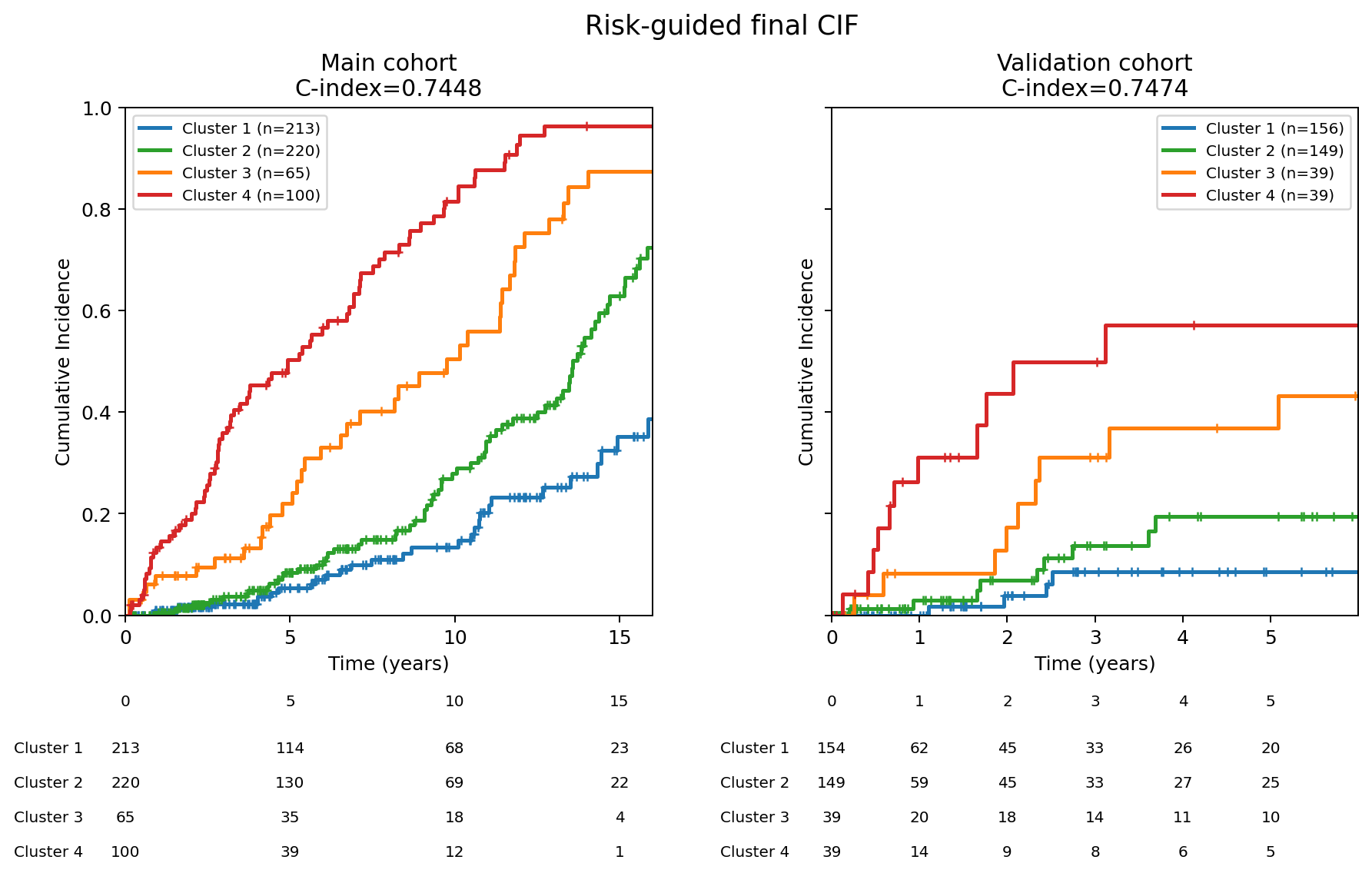
SAE cluster results after sparse-feature grouping
5-year CIF ladder
Cluster
Interpretation
Main
Validation
C1
Preserved cardiopulmonary phenotype
5.3%
8.5%
C2
Chronic anemia with early LA loading
8.4%
19.4%
C3
Anemia-driven high-output remodeling
22.0%
36.9%
C4
Cardio-renal-pulmonary vasculopathy
50.3%
57.1%
SAE main C-index
0.7448
SAE validation C-index
0.7474
Read left to right: residual state to sparse SAE features, clinically similar features to clusters, then clusters audited by baseline phenotype and 5-year CIF.
SAE analysis
Clusters are phenotype hypotheses generated from sparse hidden-state features.
From sparse latent signals to clinician-readable explanations
Every generated explanation should be anchored to active latent signals, revised when it fails, and improved with clinician feedback through reinforcement learning.
Translation
One held-out patient, two audiences: the same model evidence should survive translation.
Example patient: validation pidx=419.
Clinician-facing output
"The model predicts a cumulative incidence curve that rises modestly in the first 5 years and then plateaus, reaching ~40% by year 15."
"An anemia with right ventricular pressure overload subgroup carries lower Hemoglobin and Hematocrit but higher Estimated.RVSP and TR.Peak.Velocity; this patient sits on the activated side for anemia markers but not for RVSP/TRV. The per-patient Delta_F is +0.0009 / +0.0147 / +0.0039 / +0.0019 at 1/5/10/15y."
"A low right ventricular pressure/remodeling contrast carries lower RVSP, LV mass index, TRV, and BUN; this patient sits on all four features, with the largest positive push at 5y."
"The model predicts this patient's chance of the bad outcome starts low, about 2% by 1 year, but climbs steadily through the first five years, reaching roughly 10% by year 5."
"The curve then accelerates, jumping to about 35% by year 10, before leveling off slightly in the later years, ending near 55% by year 15."
"The strongest concern is the heart and lungs working harder than they should. The right side of the heart is under extra pressure, and the blood vessels carrying blood to the lungs are showing signs of strain."
"A secondary signal is the patient's blood counts being lower than normal, which adds a smaller but steady push to the risk, particularly in the later years."
LLM setup: judge LLM = Gemma-4-26B-A4B; two generator LLMs = Mistral-3-14B; hosted on 4xH200 NVL.
Translation
Generalizable design pattern for precision medicine
Unified does not mean one giant model for everything. It means a model family constrained by consistency across prediction, trajectory, phenotype, survival, and explanation.
Close
Take-home messages
Trajectory supervision strengthens rare-event survival prediction from baseline data.